2010년 7월 22일 목요일

Good Korean linkage analysis introduction

http://plaza.snu.ac.kr/~hokim/seminar/gene20040407.pdf

2010년 7월 21일 수요일

LD and LOD, a good tutorial

MERLIN Tutorial -- Modeling Marker-Marker Linkage Disequilibrium

This tutorial describe the procedures and options available for modeling marker-marker linkage disequilibrium with MERLIN. It assumes that you are relatively familiar with MERLIN and its standard command line options. If you haven't yet done so, it is a good idea to first learn about input file formats and non-parametric linkage analysis.

MERLIN can accomodate marker-marker linkage disequilibrium in nearly all available analyses, including parametric and non-parametric analysis of discrete traits, regression and variance-components based analysis of quantitative traits, haplotyping analyses and simulation. Modeling marker-marker linkage disequilibrium is especially important when analysing SNP linkage maps in datasets where some parental genotypes are missing. It has been shown that in these settings ignoring marker-marker linkage disequilibrium can result in severe biases in linkage calculations.

To model linkage disequilibrium, MERLIN organizes markers into clusters. Each cluster can include both SNP and microsatellite markers. MERLIN then uses population haplotype frequencies to assume linkage disequilibrium within each cluster. Two limitations of the model are that it assumes no recombination within clusters and no linkage disequilibrium between clusters. These approximations appear to be reasonable in many datasets.

For this example, we will use a simulated data set that you will find in the examples subdirectory of the MERLIN distribution or in the download page.

The dataset consists of a SNP linkage scan of a candidate chromosome in a set of 500 affected sibships, each with three genotyped affected siblings and one affected parent. The SNP data consists of clusters of 2-3 SNPs, all within 100kb of each other, genotyped approximately 5cM apart along a single chromosome (20 clusters and 59 SNPs in total).

The three standard Merlin format input files are the data file snp-scan.dat, pedigree file snp-scan.ped and map file snp-scan.map. In the pedigree file, SNP alleles 'A', 'C', 'G' and 'T' have been coded as allele 1, 2, 3 and 4, respectively. All input files are text files, and you can check their contents using the UNIX more command or using the following pedstats command:

prompt> pedstats -d snp-scan.dat -p snp-scan.ped

We are going to evaluate the evidence for linkage is this SNP data set, and a good place to start, is to run a standard non-parametric linkage analysis (--npl command option) ignoring linkage disequilibrium between markers. We will request that Merlin carry out analysis at positions spaced every 2 cM along the chromosome(--grid 2 command line option). Try running the following command:

prompt> merlin -d snp-scan.dat -p snp-scan.ped -m snp-scan.map --npl --grid 2

After the opening banner screen, your results should be similar to the following:

Phenotype: DISEASE [ALL] (500 families)
======================================================
Pos Zmean pvalue delta LOD pvalue
min -18.26 1.0 -0.408 -62.47 1.0
max 54.77 0.00000 1.225 301.0 0.00000
0.000 1.28 0.10 0.094 0.57 0.05
5.000 1.85 0.03 0.109 0.96 0.02
10.000 2.38 0.009 0.139 1.56 0.004
15.000 3.23 0.0006 0.204 3.08 0.00008
20.000 4.72 0.00000 0.308 6.75 0.00000
25.000 3.97 0.00004 0.241 4.48 0.00000
30.000 3.62 0.00014 0.234 3.98 0.00001
35.000 2.64 0.004 0.149 1.86 0.002
40.000 2.05 0.02 0.122 1.18 0.010
45.000 2.27 0.012 0.126 1.35 0.006
50.000 1.99 0.02 0.110 1.03 0.015
55.000 2.27 0.012 0.133 1.43 0.005
60.000 2.28 0.011 0.124 1.33 0.007
65.000 3.21 0.0007 0.189 2.84 0.00015
70.000 4.20 0.00001 0.236 4.62 0.00000
75.000 3.78 0.00008 0.220 3.90 0.00001
80.000 2.74 0.003 0.161 2.08 0.0010
85.000 2.23 0.013 0.127 1.34 0.006
90.000 2.20 0.014 0.127 1.33 0.007
95.000 2.28 0.011 0.154 1.66 0.003
100.000 1.87 0.03 0.187 1.65 0.003

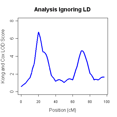
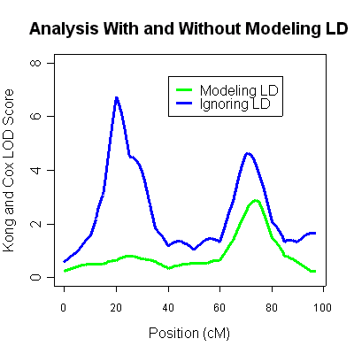
The 4th column (labeled LOD score) is the Kong and Cox LOD score for this data. You will notice two very strong LOD score peaks, one around 20cM (LOD 6.75) and another around 70cM (LOD of 4.62). Unfortunately, ignoring marker-marker LD can lead to inflated LOD scores when some parental genotypes are missing. The results are typical of situations where marker-marker disequilibrium is not modeled appropriately and should not be taken as evidence for linkage.

To verify whether there is evidence for linkage, we will repeat the previous analysis, but modeling marker-marker disequibrium. First, we will carry out analyses using pre-specified clusters and haplotype frequencies. Next, we will see how Merlin can automatically define clusters using the available marker map and genotype data.

We will use cluster definitions in the file snp-scan.clusters. This file describes clusters of SNPs in linkage disequilibrium. This file can be generated by the user, or by a previous MERLIN run. We will describe the file in detail, since it should help clarify how MERLIN models linkage disequilibrium.

The file describes a series of clusters, each consisting of a series of consecutive markers. The description of each cluster begins on a separate line with the word CLUSTER followed by a series of marker names, that must exactly match the data and map files. Optionally, this line can be followed by a series of entries, each on a separate line, describing the haplotypes in the cluster and their frequencies. Each of these lines begins with the word HAPLO followed by a haplotype frequency and a series of alleles.

For example, this is the first cluster in the snp-scan.clusters file:

CLUSTER rs556990 rs553316 rs7989953
HAPLO 0.4500 3 2 1
HAPLO 0.3167 3 2 3
HAPLO 0.2000 1 4 1
HAPLO 0.0333 1 4 3

The cluster includes three markers (rs556990, rs553316, rs7989953) organized into 4 distinct haplotypes. The first two markers are in complete linkage disequilibrium, such that allele 3 at rs556990 always appears with allele 2 at rs553316, whereas allele 1 at rs556990 always appears with allele 4 at rs553316. The last marker is in strong, but incomplete disequilibrium with the first two: allele 3 for rs7989953 nearly always occurs on the 3-2 haplotype for markers rs556990 and rs553316.

After reading the file with clustering information, MERLIN will do the following:

* Check that all markers within a cluster are contiguous. If they are not, you will get an error message.
* Check that all markers within a cluster map to the same genetic map position. If they do not, Merlin will nudge their positions to ensure the within cluster recombination rate is zero.
* If haplotype frequency estimates are not provided, they will be calculated using the available genotype data and a maximum-likelihood E-M algorithm.

So let's repeat the original analysis, but modeling of marker-marker disequilibrium enabled. To do this, use the following command-line:

prompt> merlin -d snp-scan.dat -p snp-scan.ped -m snp-scan.map --npl --grid 5 --cluster snp-scan.clusters

After the opening banner screen, you will first see a series of information messages:

MARKER CLUSTERS: Marker map changed, see [merlin-clusters.log]
MARKER CLUSTERS: User supplied file defines 20 clusters

Family: 101 - Founders: 2 - Descendants: 3 - Bits: 4
Cluster at marker rs7334521 dropped [OBLIGATE RECOMBINANT]

Family: 287 - Founders: 2 - Descendants: 3 - Bits: 4
Cluster at marker rs7334521 dropped [UNKNOWN HAPLOTYPE]

The first two lines indicate that the cluster information was successfully loaded. Since MERLIN assumes no recombination within clusters, the original genetic map was adjusted slightly -- you can examine the contents of merlin-clusters.log for details. In addition, MERLIN encountered two families (101 and 287) where genotypes for one cluster did not fit with the model described in the clustering file. In family 101, the observed genotypes imply an obligate recombinant in the cluster including markers rs7334521, rs4495999 and rs9546406. In family 287, the observed genotypes imply a haplotype that is not present in the clustering file. In both families, genotypes for markers rs7334521, rs4495999 and rs9546406 will be marked as missing to allow analysis to proceed. In our experience, discarding a small proportion of the available genotypes in this manner results in no noticeable biases.

After these messages, you will find the linkage analysis results, which should be similar to the following:

Phenotype: DISEASE [ALL] (500 families)
======================================================
Pos Zmean pvalue delta LOD pvalue
min -18.26 1.0 -0.408 -62.47 1.0
max 54.77 0.00000 1.225 301.0 0.00000
0.011 0.82 0.2 0.061 0.24 0.15
5.011 1.17 0.12 0.070 0.39 0.09
10.011 1.32 0.09 0.078 0.49 0.07
15.011 1.31 0.09 0.083 0.52 0.06
20.011 1.43 0.08 0.098 0.67 0.04
25.011 1.66 0.05 0.107 0.84 0.02
30.011 1.54 0.06 0.102 0.75 0.03
35.011 1.47 0.07 0.085 0.60 0.05
40.011 1.10 0.14 0.067 0.35 0.10
45.011 1.30 0.10 0.074 0.46 0.07
50.011 1.41 0.08 0.079 0.53 0.06
55.011 1.37 0.09 0.081 0.53 0.06
60.011 1.57 0.06 0.087 0.65 0.04
65.011 2.26 0.012 0.136 1.44 0.005
70.011 3.05 0.0011 0.178 2.55 0.0003
75.011 3.24 0.0006 0.192 2.92 0.00012
80.011 2.34 0.010 0.138 1.53 0.004
85.011 1.74 0.04 0.099 0.82 0.03
90.011 1.45 0.07 0.084 0.58 0.05
95.011 0.88 0.2 0.060 0.25 0.14

There is now a single linkage peak around 75cM (LOD of 2.92). The original peak around 20cM has completely disappeared, and was simply an artifact of linkage disequilibrium between markers. Thus, there is some good evidence for a single linkage peak in these data (at around 75cM). The analysis ignoring linkage disequilibrium, which showed an additional peak at around 20cM was quite inaccurate.

If you want to model linkage disequilibrium, but do not have a file describing preset clusters for your SNP mapping panel, MERLIN provides two options for automatically clustering markers. The --distance k option inserts a cluster breakpoint between markers that are less than k cM apart (that is, all consecutive markers spaced less than k cM are placed into a cluster). The --rsq treshold option calculates pairwise r2 between neighboring markers and creates a cluster joining markers for which pairwise r2 > threshold and all intervening markers.

To explore these alternative options, try the following command lines:

prompt> merlin -d snp-scan.dat -p snp-scan.ped -m snp-scan.map --npl --grid 5 --rsq 0.1 --cfreq
prompt> merlin -d snp-scan.dat -p snp-scan.ped -m snp-scan.map --npl --grid 5 --dist 3 --cfreq
prompt> merlin -d snp-scan.dat -p snp-scan.ped -m snp-scan.map --npl --grid 5 --clusters snp-scan.clusters-only --cfreq

The first command-line, will search for markers for which r2 is > 0.10 and define clusters including each identified pair and the intervening markers. The second command-line will group markers that are less than 3 cM apart into a cluster. The final command-line will use the cluster definitions in the snp-scan.clusters-only file, but estimate haplotype frequencies from the available genotype data. In each case, the --cfreq flag requests that the estimated clusters and their frequencies should be saved to a file.

That is it! You should be on your way to modeling linkage disequilibrium between markers in your own data, so as to make the best use of available SNP mapping panels.

To learn about other analyses options, you might want to check the non-parametric linkage analysis or parametric linkage analysis sections, or proceed haplotyping, simulation or ibd estimation sections.

LD, linkage dis-equilibrium from wikipedia

Linkage disequilibrium

From Wikipedia, the free encyclopedia

Jump to: navigation, search

This article may require cleanup to meet Wikipedia's quality standards. Please improve this article if you can. (September 2009)

"Graph depicting evolution of linkage disequilibrium in a haploid population with positive assortative mating (inbreeding); graph shows the trajectories of 1,024 populations with randomly generated initial allele frequencies; trajectories beginning close to 0 slope away from 0 sharply then decline to 0 asymptotically, while trajectories beginning near 0 diminish to 0"

Depiction of evolution of linkage disequilibrium in randomly-generated simulated haploid populations with positive assortative mating

In population genetics, linkage disequilibrium is the non-random association of alleles at two or more loci, not necessarily on the same chromosome. It is not the same as linkage, which describes the association of two or more loci on a chromosome with limited recombination between them. Linkage disequilibrium describes a situation in which some combinations of alleles or genetic markers occur more or less frequently in a population than would be expected from a random formation of haplotypes from alleles based on their frequencies. Non-random associations between polymorphisms at different loci are measured by the degree of linkage disequilibrium (LD). Numerically, it is the difference between observed and expected (assuming random distributions) allelic frequencies.

An example is the prevalence of two rare diseases in Finland: there, compared to elsewhere in Europe, cystic fibrosis is less prevalent but congenital chloride diarrhea is more prevalent (see Finnish disease heritage). Both diseases are due to mutations on chromosome 7, in adjacent genes.^[1]

The level of linkage disequilibrium is influenced by a number of factors including genetic linkage, selection, the rate of recombination, the rate of mutation, genetic drift,non-random mating, and population structure. For example, some organisms (such as bacteria) may show linkage disequilibrium because they reproduce asexually and there is no recombination to break down the linkage disequilibrium.

[hide]

[edit] Linkage disequilibrium measure, D

If we look at haplotypes for two loci A and B with two alleles each—a two-locus, two-allele model—the following table denotes the frequencies of each combination:

Haplotype	Frequency
$A 1 B 1$	$x 11$
$A 1 B 2$	$x 12$
$A 2 B 1$	$x 21$
$A 2 B 2$	$x 22$

Note that these are relative frequencies. One can use the above frequencies to determine the frequency of each of the alleles:

Allele	Frequency
$A 1$	$p 1 = x 11 + x 12$
$A 2$	$p 2 = x 21 + x 22$
$B 1$	$q 1 = x 11 + x 21$
$B 2$	$q 2 = x 12 + x 22$

If the two loci and the alleles are independent from each other, then one can express the observation $A 1 B 1$ as " $A 1$ is found and $B 1$ is found". The table above lists the frequencies for $A 1$ , $p 1$ , and for $B 1$ , $q 1$ , hence the frequency of $A 1 B 1$ is $x 11$ , and according to the rules of elementary statistics $x 11 = p 1 q 1$ .

The deviation of the observed frequency of a haplotype from the expected is a quantity^[2] called the linkage disequilibrium^[3] and is commonly denoted by a capital D:

D = x 11 - p 1 q 1

In the genetic literature the phrase "two alleles are in LD" usually means that $D \ne 0$ . Contrariwise, "linkage equilibrium" denotes the case $D = 0$ .

The following table illustrates the relationship between the haplotype frequencies and allele frequencies and D.

	$A 1$	$A 2$	Total
$B 1$	$x 11 = p 1 q 1 + D$	$x 21 = p 2 q 1 - D$	$q 1$
$B 2$	$x 12 = p 1 q 2 - D$	$x 22 = p 2 q 2 + D$	$q 2$
Total	$p 1$	$p 2$	$1$

$D$ is easy to calculate with, but has the disadvantage of depending on the frequency of the alleles. This is evident since frequencies are between 0 and 1. There can be no $D$ observed if any locus has an allele frequency 0 or 1 and is maximal when frequencies are at 0.5. Lewontin (1964) suggested normalising D by dividing it with the theoretical maximum for the observed allele frequencies. Thus $D'=\frac{D}{D_\max}$ when $D \ge 0$ When $D'=\frac{D}{D_\min}$

$D max$ is given by the smaller of $p 1 q 2$ and $p 2 q 1$ . $D min$ is given by the larger of $- p 1 q 1$ and $- p 2 q 2$

Another measure of LD which is an alternative to D' is the correlation coefficient between pairs of loci, denoted as $r=\frac{D}{\sqrt{p_1p_2q_1q_2}}$ . This is also adjusted to the loci having different allele frequencies. There is some relationship between $r$ and $D'.$ ^[4]

In summary, linkage disequilibrium reflects the difference between the expected haplotype frequencies under the assumption of independence, and observed haplotype frequencies. A value of 0 for D' indicates that the examined loci are in fact independent of one another, while a value of 1 demonstrates complete dependency.

[edit] Role of recombination

In the absence of evolutionary forces other than random mating and Mendelian segregation, the linkage disequilibrium measure $D$ converges to zero along the time axis at a rate depending on the magnitude of the recombination rate $c$ between the two loci.

Using the notation above, $D = x 11 - p 1 q 1$ , we can demonstrate this convergence to zero as follows. In the next generation, $x 11'$ , the frequency of the haplotype $A 1 B 1$ , becomes

$x_{11}' = (1-c)\,x_{11} + c\,p_1 q_1$

This follows because a fraction $(1 - c)$ of the haplotypes in the offspring have not recombined, and are thus copies of a random haplotype in their parents. A fraction $x 11$ of those are $A 1 B 1$ . A fraction $c$ have recombined these two loci. If the parents result from random mating, the probability of the copy at locus $A$ having allele $A 1$ is $p 1$ and the probability of the copy at locus $B$ having allele $B 1$ is $q 1$ , and as these copies are initially on different haplotypes, these are independent events so that the probabilities can be multiplied.

This formula can be rewritten as

$x_{11}' - p_1 q_1 = (1-c)\,(x_{11} - p_1 q_1)$

so that

$D_1 = (1-c)\;D_0$

where $D$ at the $n$ -th generation is designated as $D n$ . Thus we have

$D_n = (1-c)^n\; D_0$ .

If $n \to \infty$ , then $(1-c)^n \to 0$ so that $D n$ converges to zero.

If at some time we observe linkage disequilibrium, it will disappear in future due to recombination. However, the smaller the distance between the two loci, the smaller will be the rate of convergence of $D$ to zero.

[edit] Linkage disequilibrium appears frequently in genetic systems

[edit] Human leucocyte antigen (HLA)

HLA constitutes a group of cell surface antigens as MHC of humans. Because HLA genes are located at adjacent loci on the particular region of a chromosome and presumed to exhibit epistasis with each other or with other genes, a sizable fraction of alleles are in linkage disequilibrium.

An example of such linkage disequilibrium is between HLA-A1 and B8 alleles in unrelated Danes^[5] referred to by Vogel and Motulsky (1997).^[6]

Table 1. Association of HLA-A1 and B8 in unrelated Danes^[5]
			Antigen j		Total
			No. of individuals
			$+$	$-$
			$B 8 +$	$B 8 -$
Antigen i	$+$	$A 1 +$	$a = 376$	$b = 237$	$C$
Antigen i	$-$	$A 1 -$	$c = 91$	$d = 1265$	$D$
Total			$A$	$B$	$N$

Because HLA is codominant and HLA expression is only tested locus by locus in surveys, LD measure is to be estimated from such a 2x2 table to the right.^[6]^[7]^[8]^[9]

p f i = frequency of antigen i = C / N = 0.311

p f j = 0.237

$gf_i=\text{frequency of gene }i=1-\sqrt{1-pf_i}=0.170$ ,

and

$hf_{ij}=\text{estimated frequency of haplotype }ij=gf_i\; gf_j=0.0215$ .

Denoting the '―' alleles at antigen i to be 'x,' and at antigen j to be 'y,' the observed frequency of haplotype xy is

$o[hf_{xy}]=\sqrt{d/N}$

and the estimated frequency of haplotype xy is

$e[hf_{xy}]=\sqrt{(D/N)(B/N)}$ .

Then LD measure $Δ i j$ is expressed as

$\Delta_{ij}=o[hf_{xy}]-e[hf_{xy}]=\frac{\sqrt{Nd}-\sqrt{BD}}{N}=0.0769$ .

Standard errors $S E s$ are obtained as follows:

$SE\text{ of }gf_i=\sqrt{C}/(2N)=0.00628$ ,

$SE\text{ of }hf_{ij}=\sqrt{\frac{(1-\sqrt{d/B})(1-\sqrt{d/D})-hf_{ij}-hf_{ij}^2/2}{2N}}=0.00514$

$SE\text{ of }\Delta_{ij}=\frac{1}{2N}\sqrt{a-4N\Delta_{ij}\left (\frac{B+D}{2\sqrt{BD}}-\frac{\sqrt{BD}}{N}\right )}=0.00367$ .

Then, if

t = Δ i j / (S E of Δ i j)

exceeds 2 in its absolute value, the magnitude of $Δ i j$ is large statistically significantly. For data in Table 1 it is 20.9, thus existence of statistically significant LD between A1 and B8 in the population is admitted.

Table 2. Linkage disequilibrium among HLA alleles in Caucasians^[9]
HLA-A alleles i	HLA-B alleles j	$Δ i j$	$t$
A1	B8	0.065	16.0
A3	B7	0.039	10.3
A2	Bw40	0.013	4.4
A2	Bw15	0.01	3.4
A1	Bw17	0.014	5.4
A2	B18	0.006	2.2
A2	Bw35	-0.009	-2.3
A29	B12	0.013	6.0
A10	Bw16	0.013	5.9

Table 2 shows some of the combinations of HLA-A and B alleles where significant LD was observed among Caucasians.^[9]

Vogel and Motulsky (1997)^[6] argued how long would it take that linkage disequilibrium between loci of HLA-A and B disappeared. Recombination between loci of HLA-A and B was considered to be of the order of magnitude 0.008. We will argue similarly to Vogel and Motulsky below. In case LD measure was observed to be 0.003 in Caucasians in the list of Mittal^[9] it is mostly non-significant. If $Δ 0$ had reduced from 0.07 to 0.003 under recombination effect as shown by $Δ n = (1 - c) n Δ 0$ , then $n\approx 400$ . Suppose a generation took 25 years, this means 10,000 years. The time span seems rather short in the history of humans. Thus observed linkage disequilibrium between HLA-A and B loci might indicate some sort of interactive selection.^[6]

Further information: HLA A1-B8 haplotype

[edit] Between an HLA locus and a presumed major gene locus having disease susceptibility

Presence of linkage disequilibrium between an HLA locus and a presumed major gene of disease susceptibility corresponds to any of the following phenomena:

Relative risk for the person having a specific HLA allele to become suffered from a particular disease is larger than one.^[10]
The HLA antigen frequency among patients exceeds more than that among a healthy population. This is evaluated by $δ$ value^[11] to exceed 0.

Table 3. Association of ankylosing spondylitis with HLA-B27 allele^[12]
		Patients	Healthy controls	Total
		Ankylosing spondylitis		Total
HLA alleles	$B 27 +$	$a = 96$	$b = 77$	$C$
HLA alleles	$B 27 -$	$c = 22$	$d = 701$	$D$
Total		$A$	$B$	$N$

2x2 association table of patients and healthy controls with HLA alleles shows a significant deviation from the equilibrium state deduced from the marginal frequencies.

(1) Relative risk

Relative risk of an HLA allele for a disease is approximated by the odds ratio in the 2x2 association table of the allele with the disease. Table 3 shows association of HLA-B27 with ankylosing spondylitis among a Dutch population.^[12] Relative risk $x$ of this allele is approximated by

$x=\frac{a/b}{c/d}=\frac{ad}{bc}\;(=39.7,\text{ in Table 3 })$ .

Woolf's method^[13] is applied to see if there is statistical significance. Let

$y=\ln (x)\;(=3.68)$

and

$\frac{1}{w}=\frac{1}{a}+\frac{1}{b}+\frac{1}{c}+\frac{1}{d}\;(=0.0703)$ .

Then

$\text{[math]}$ \chi^2(p=0.001,\; df=1)=10.8 \right ]" src="http://upload.wikimedia.org/math/3/8/8/388430d3c9392e03a17d8f42665f3347.png">

follows the chi-square distribution with $d f = 1$ . In the data of Table 3, the significant association exists at the 0.1% level. Haldane's^[14] modification applies to the case when either of $a,\; b,\;c,\text{ and }d$ is zero, where replace $x$ and $1 / w$ with

$x=\frac{(a+1/2)(d+1/2)}{(b+1/2)(c+1/2)}$

and

$\frac{1}{w}=\frac{1}{a+1}+\frac{1}{b+1}+\frac{1}{c+1}+\frac{1}{d+1}$ ,

respectively.

Table 4. Association of HLA alleles with rheumatic and autoimmune diseases among white populations^[10]
Disease	HLA allele	Relative risk (%)	FAD (%)	FAP (%)	$δ$
Ankylosing spondylitis	B27	90	90	8	0.89
Reiter's syndrome	B27	40	70	8	0.67
Spondylitis in inflammatory bowel disease	B27	10	50	8	0.46
Rheumatoid arthritis	DR4	6	70	30	0.57
Systemic lupus erythematosus	DR3	3	45	20	0.31
Multiple sclerosis	DR2	4	60	20	0.5
Diabetes mellitus type 1	DR4	6	75	30	0.64

In Table 4, some examples of association between HLA alleles and diseases are presented.^[10]

(1a) Allele frequency excess among patients over controls

Even high relative risks between HLA alleles and the diseases were observed, only the magnitude of relative risk would not be able to determine the strength of association.^[11] $δ$ value is expressed by

$\delta=\frac{FAD-FAP}{1-FAP},\;\;0\le \delta \le 1$ ,

where $F A D$ and $F A P$ are HLA allele frequencies among patients and healthy populations, respectively.^[11] In Table 4, $δ$ column was added in this quotation. Putting aside 2 diseases with high relative risks both of which are also with high $δ$ values, among other diseases, juvenile diabetes mellitus (type 1) has a strong association with DR4 even with a low relative risk $= 6$ .

(2) Discrepancies from expected values from marginal frequencies in 2x2 association table of HLA alleles and disease

This can be confirmed by $χ 2$ test calculating

$\chi^2=\frac{(ad-bc)^2 N}{ABCD}\;(=336,\text{ for data in Table 3; }P<0.001)$ .

where $d f = 1$ . For data with small sample size, such as no marginal total is greater than 15 (and consequently $N \le 30$ ), one should utilize Yates' correction for continuity or Fisher's exact test.^[15]

[edit] Resources

A comparison of different measures of LD is provided by Devlin & Risch ^[16]

The International HapMap Project enables the study of LD in human populations online. The Ensembl project integrates HapMap data and such from dbSNP in general with other genetic information.

[edit] Analysis software

LDHat
Haploview
LdCompare^[17] — open-source software for calculating LD.
PyPop
SNP and Variation Suite - commercial software with interactive LD plot.
GOLD - Graphical Overview of Linkage Disequilibrium
TASSEL - software to evaluate linkage disequilibrium, traits associations, and evolutionary patterns

[edit] Simulation software

Haploid — a C library for population genetic simulation (GPL)

[edit] See also

[edit] References

^ Höglund P, Haila S, Socha J, Tomaszewski L, Saarialho-Kere U, Karjalainen-Lindsberg ML, Airola K, Holmberg C, de la Chapelle A, Kere J (November 1996). "Mutations of the Down-regulated in adenoma (DRA) gene cause congenital chloride diarrhoea". Nature Genetics 14 (3): 316–9. doi:10.1038/ng1196-316. PMID 8896562.
^ Robbins, R.B. (1 July 1918). "Some applications of mathematics to breeding problems III". Genetics 3 (4): 375–389. PMID 17245911. PMC 1200443. http://www.genetics.org/cgi/reprint/3/4/375.
^ R.C. Lewontin and K. Kojima (1960). "The evolutionary dynamics of complex polymorphisms". Evolution 14 (4): 458–472. doi:10.2307/2405995. http://links.jstor.org/sici?sici=0014-3820%28196012%2914%3A4%3C458%3ATEDOCP%3E2.0.CO%3B2-4.
^ P.W. Hedrick and S. Kumar (2001). "Mutation and linkage disequilibrium in human mtDNA". Eur. J. Hum. Genet. 9 (12): 969–972. doi:10.1038/sj.ejhg.5200735. PMID 11840186.
^ ^a ^b Svejgaard A, Hauge M, Jersild C, Plaz P, Ryder LP, Staub Nielsen L, Thomsen M (1979). The HLA System: An Introductory Survey, 2nd ed. Basel; London; Chichester: Karger; Distributed by Wiley, ISBN 3805530498(pbk).
^ ^a ^b ^c ^d Vogel F, Motulsky AG (1997). Human Genetics : Problems and Approaches, 3rd ed. Berlin; London: Springer, ISBN 3540602909.
^ Mittal KK, Hasegawa T, Ting A, Mickey MR, Terasaki PI (1973). "Genetic variation in the HL-A system between Ainus, Japanese, and Caucasians," In Dausset J, Colombani J, eds. Histocompatibility Testing, 1972, pp. 187-195, Copenhagen: Munksgaard, ISBN 8716011015.
^ Yasuda N, Tsuji K (1975). "A counting method of maximum likelihood for estimating haplotype frequency in the HL-A system." Jinrui Idengaku Zasshi 20(1): 1-15, PMID 1237691.
^ ^a ^b ^c ^d Mittal KK (1976). "The HLA polymorphism and susceptibility to disease." Vox Sang 31: 161-173, PMID 969389.
^ ^a ^b ^c Gregersen PK (2009). "Genetics of rheumatic diseases," In Firestein GS, Budd RC, Harris ED Jr, McInnes IB, Ruddy S, Sergent JS, eds. (2009). Kelley's Textbook of Rheumatology, pp. 305-321, Philadelphia, PA: Saunders/Elsevier, ISBN 9781416032854.
^ ^a ^b ^c Bengtsson BO, Thomson G (1981). "Measuring the strength of associations between HLA antigens and diseases." Tissue Antigens 18(5): 356-363, PMID 7344182.
^ ^a ^b Nijenhuis LE (1977). "Genetic considerations on association between HLA and disease." Hum Genet 38(2): 175-182, PMID 908564.
^ Woolf B (1955). "On estimating the relation between blood group and disease." Ann Hum Genet 19(4): 251-253, PMID 14388528.
^ Haldane JB (1956). "The estimation and significance of the logarithm of a ratio of frequencies." Ann Hum Genet 20(4): 309-311, PMID 13314400.
^ Sokal RR, Rohlf FJ (1981). Biometry: The Principles and Practice of Statistics in Biological Research. Oxford: W.H. Freeman, ISBN 0716712547.
^ Devlin B., Risch N. (1995). "A Comparison of Linkage Disequilibrium Measures for Fine-Scale Mapping". Genomics 29 (2): 311–322. doi:10.1006/geno.1995.9003. PMID 8666377. http://www.sciencedirect.com/science?_ob=MImg&_imagekey=B6WG1-45S9156-30-1&_cdi=6809&_user=128590&_orig=browse&_coverDate=09%2F30%2F1995&_sk=999709997&view=c&wchp=dGLbVtb-zSkzk&md5=71c2158ad4c51ae80b12a68c68814f78&ie=/sdarticle.pdf.
^ Hao K., Di X., Cawley S. (2007). "LdCompare: rapid computation of single- and multiple-marker r2 and genetic coverage". Bioinformatics 23 (2): 252–254. doi:10.1093/bioinformatics/btl574. PMID 17148510. http://bioinformatics.oxfordjournals.org/cgi/reprint/23/2/252.

[edit] Further reading

Hedrick, Philip W. (2005). Genetics of Populations (3rd ed.). Sudbury, Boston, Toronto, London, Singapore: Jones and Bartlett Publishers. ISBN 0763747726.
Bibliography: Linkage Disequilibrium Analysis : a bibliography of more than one thousand articles on Linkage disequilibrium published since 1918.

[hide] v • d • e Topics in population genetics

Key concepts	Hardy-Weinberg law · Genetic linkage · Linkage disequilibrium · Fisher's fundamental theorem · Neutral theory · Price equation

Selection	Natural · Sexual · Artificial · Ecological

Effects of selection on genomic variation	Genetic hitchhiking · Background selection

Genetic drift	Small population size · Population bottleneck · Founder effect · Coalescence · Balding–Nichols model

Founders	R. A. Fisher · J. B. S. Haldane · Sewall Wright

Related topics	Evolution · Microevolution · Evolutionary game theory · Fitness landscape · Genetic genealogy

List of evolutionary biology topics

GWA study: How to read a genome-wide association study

How to read a genome-wide association study

18/07/2010
Categories: Background
Written by Jeff Barrett

As any avid follower of genomics or medical genetics knows, genome-wide association studies (GWAS) have been the dominant tool used by complex disease genetics researchers in the last five years. There’s a very active debate in the field about whether GWAS have revolutionized our understanding of disease genetics or whether they were a waste of money for little tangible gain. No matter where you fall in that spectrum, however, you need only to browse the table of contents of any recent issue of Nature Genetics to see how ubiquitous they are. Since GWAS provide so much of the fodder for unzipping your genome, and in order to help you cut through the hype in the mainstream press coverage of GWAS, I’ve put together a quick primer on how to go straight to the original paper and decide for yourself whether it’s a landmark finding or a dud.

The basic GWAS approach is to look at approximately a million positions in the human genome (called ‘SNPs’) where different people carry different versions of the genetic code (so at some particular position I might have an ‘A’ and you might have a ‘C’). I’m going to focus here on the most common GWAS design, called case-control, where the goal is to compare the frequencies of these different versions between a group of healthy individuals (controls) and another group of people with a specific disease (cases). The places where the frequencies between cases and controls are significantly different are therefore associated with risk of developing the disease.

It’s not always that easy, though! Listed below are five issues raised by almost every GWAS and how you can try to zero in on the key details about them in the paper. A few example figures are taken from the WTCCC GWAS, which also serves (in my biased view!) as an excellent example of the right way to carry out one of these studies.

Sample size. One key thing to look for early in the paper is how many samples the study has managed to collect. GWAS are generally aimed at finding very small effects (increasing your risk by, say, 15%) so they need lots of samples to confirm such small differences with statistical confidence. If a paper has fewer than a thousand cases and controls you should be suspicious. There are some exceptions (like big genetic effects on severe side effects from drugs), but these are rare.
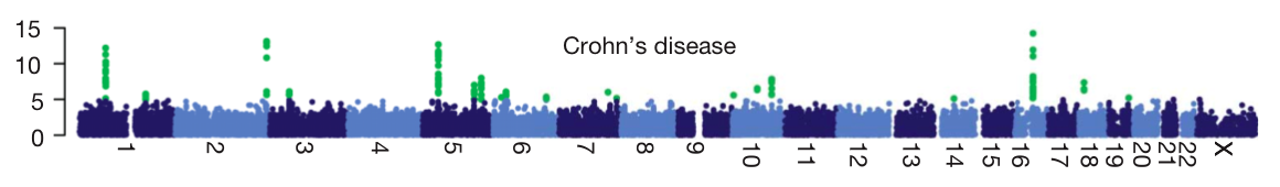
Quality control. The biggest challenge to successfully carrying out a GWAS is getting good, clean genotype data. Pay close attention not only to the standard QC metrics (genotype call rate, Hardy-Weinberg equilibrium, etc) but also to whether extra attention was focused on the genotypes of the most associated SNPs. Most GWAS practitioners go to great lengths to find lab problems that might create false positive associations, but even after years of these best practices being understood, there are sometimes still GWAS published where authors, reviewers and journal have all missed possible genotype QC issues. Good QC should filter out artifacts, and yield a ‘manhattan plot’ like the one below. Each point is a SNP laid out across the human chromosomes from left to right, and the heights correspond to the strength of the association to disease. You’ll see that the strongest associations (highlighted in green) form neat peaks where nearby correlated SNPs all show the same signal. Any manhattan plot with points all over the place should be viewed as highly suspicious (as raised by Daniel in this excellent post).
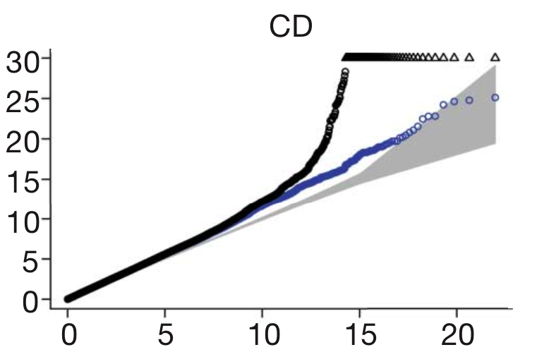
Confounders. Be on the lookout for any variable in the study which could be different between cases and controls other than the disease itself. For instance, if the disease is more common in one part of the world than another, and this effect isn’t accounted for, then the naturally arising genetic differences between those groups of people will look like they’re associated with disease. This ‘population structure’, as it’s called, is the most commonly discussed confounder, but many others exist, such as whether cases and controls were genotyped in the same laboratory, or the DNA was collected by the same method.One statistical tool, called the ‘QQ plot’ is a common way for GWAS to show that confounders aren’t at work. The QQ plot shows the expected distribution of association test statistics (X-axis) across the million SNPs compared to the observed values (Y-axis). Any deviation from the X=Y line implies a consistent difference between cases and controls across the whole genome (suggesting a bias like the ones I’ve mentioned). A clean QQ plot (see below), on the other hand, should show a solid line matching X=Y until it sharply curves at the end (representing the small number of true associations among thousands of unassociated SNPs). The blue points in this figure show what’s left after removing the validated associations, which shows that most of that tail was, in fact, due to true disease variants, but also that more interesting results might still be lurking in the data.
Replication. The ultimate arbiter of a GWAS result is whether it can be replicated independently. It’s important to remember that this doesn’t just mean independent samples (though that’s crucial) but also using an independent technology. That way, any QC problems or confounders which affected the original study won’t affect the replication.
Biology. Given that a GWAS has some firm results, there’s almost always some speculative comment about why these regions of the genome are important to this disease. Take this section with a grain of salt, since it’s surprisingly easy to dig up a paper published at some point in history to support almost any functional hypothesis!

Tags: GWAS.
4 Comments

4 Responses to “How to read a genome-wide association study”

Feed for this Entry Trackback Address

Dan Frost
19/07/2010 at 14:58

You make some very good points about factors that can take the magic out of a GWAS or lead to fantastic but untrue findings. Sample size is a big one, but its effect can be mitigated by a well defined pedigree structure.

In our experience we have found quality control on the front end (in study design) and on the back end (standard statistical corrections) to be something of an “elephant in the room” for SNP and, particularly, CNV genome-wide studies.

We did a webcast on the subject about a year ago linked below.

http://www.goldenhelix.com/Events/recordings/study-design/index.html

Great post!
Susan Colilla
19/07/2010 at 18:03

Thanks for sharing the information on how to assess the quality of a GWAS study. In epidemiology (genetic or otherwise), this needs to be done on a regular basis. Many of the same factors important for a quality GWAS also hold true for high quality non-genetic epidemiolgoic studies such as: sample size, study design, confounding/bias (uncontrolled structure in population) and phenotype/exposure definition. It is also important to keep in mind study differences when combining results into a meta-analysis.
Keep up the good work!
Wes Conard
21/07/2010 at 16:02

Great post and great writing. This kind of format–lots of perspective and background, practical advice, examples that are easy to follow–is really helpful in understanding these issues. I encourage you to continue to write at this “level” so that your ideas are accessible to everyone. -W
Vijai Joseph
21/07/2010 at 18:57

Nice intro to GWAS. I think a little more elaboration on the population stratification issues, use of PCA to correct for correlated SNPs, time to event analysis, issues of age matching in some instances can be added.

However, the most important lacunae I see is the interpretation of results. A concise summary of OR, HR, GRR and PAF may be useful. Considering the title of the article, I believe that is a required ingredient.
Cheers
JVJ

bioanthropology